What Are Expected Goals (xG)?

Data and statistics have become far more prevalent in football over recent years. At the forefront of this is expected goals (or xG). Since xG was introduced in 2012 by Opta’s Sam Green, the metric has gone on to become one of the most widespread and insightful within football analytics.

Following early adoption in the betting and pro markets, expected goals has now become a regular feature for mainstream broadcasters such as Sky Sports and BBC’s Match of the Day. xG has ascended from the laptops of analysts and now regularly finds itself in the mouths of Premier League managers. Liverpool’s Jurgen Klopp recently compared their expected goals output to Manchester City while Aston Villa’s Dean Smith often used the metric in interviews this season to discuss his team’s underlying performances.

Expected goals is one of the first advanced metrics to become widely known amongst general football fans and so it has inevitably faced its critics over the years (see Jeff Stelling in 2017). A battle between the traditional way of viewing the game and the upcoming world of data analytics. However, before we pass our judgement, it is important to understand how the metric works and how we should be using it.

What Are Expected Goals (xG)?

Expected goals (or xG) measures the quality of a chance by calculating the likelihood that it will be scored from a particular position on the pitch during a particular phase of play. This value is based on several factors from before the shot was taken. xG is measured on a scale between zero and one, where zero represents a chance that is impossible to score and one represents a chance that a player would be expected to score every single time.

We know that a chance from the halfway line isn’t as likely to result in a goal as a chance from inside the box. With xG, we can actually quantify how likely a player is to score from each of these situations. For example, suppose the chance from inside the box with a given set of pre-shot characteristics was worth 0.1 xG. This means that an average player would be expected to score one goal from every ten shots in this situation or 10% of the time.

The terminology may be new, but these phrases have been used by football fans and commentators for years before xG was introduced – “he scores that nine times out of ten” or “he should’ve had a hat-trick”.

Common Misconceptions

The main criticisms of expected goals (xG) often appear in scenarios where the metric isn’t actually being applied correctly. The most common of which is at the game level. The team that has the higher xG in a match doesn’t necessarily imply that they should’ve won the game. xG is only measuring chance quality and not the expected outcome of the game. Exactly as the old saying suggests, goals do change games and the score line influences how teams play. If a team takes an early lead, they don’t necessarily ‘need’ to generate more chances and we often expect to see the opposition generate more goal scoring opportunities for the remainder of the game in pursuit of a comeback.

Another misconception is in the literal interpretation of the metric name. We do not “expect” goals to occur exactly as the likelihood predicts. We also understand that fractions of goals cannot be scored. The name “expected goals” is derived from the mathematical concept of “expected value” and it is a measure of the likelihood of an outcome occurring. The expected value of a fair coin toss is 50% likely to land on heads and 50% likely to land on tails (the expected heads or the expected tails is 0.5). We do not expect exactly half of our tosses to land on each outcome, but rather that over a larger number of coin tosses, it is likely to regress to this balance. The same applies to expected goals. Variance from the expected value is inevitable and this is valuable information that we can analyse in football.

A player or team who has been overperforming their xG, does not then have to underperform to regress to expectation. This is a concept known as the Gambler’s Fallacy. While we would expect them to regress back to scoring in line with their expectation with their future shots, they have already ‘banked’ this overperformance and so we will still expect them to overperform by this amount in the season aggregates. In the same way, if a coin toss landed on heads ten times in a row, future coin tosses are still equally likely to land on heads as they are tails, but the ten times that the coin landed on heads have already happened.

How Do We Calculate Expected Goals?

While watching a game, we can intuitively tell which chances were more or less likely to be scored. How close was the shooter to goal? Were they shooting from a good angle? Was it a one-on-one? Was it a header?

The difficulty is that there are an average of 25 shots per game that we need to work this out for, all potentially from unique situations. The advantage of our expected goals model is that we can now take the variables above – and others – and quantify how each of these affects the likelihood of a goal being scored. With this, it allows us to value the quality of the chances for all 9,398 shots taken in the Premier League 2019-20 season in a matter of seconds.

Stats Perform’s xG model is built using a logistic regression model that is powered by hundreds of thousands of shots from our historical Opta data and incorporates a number of variables that affect the likelihood of a goal being scored, some of the most important of which are listed below:

• Distance to the goal
• Angle to the goal​
• One-on-one
• Big chance
• Body part (e.g., header or foot)
• Type of assist (e.g., through ball, cross, pull-back etc) ​
• Pattern of play (e.g., open play, fast break, direct free kick, corner kick, throw-in etc)

We​ recognise that some situations are particularly unique and so these are modelled independently. Penalties are given a constant value corresponding to their overall conversion rate (0.79 xG); direct free kicks have their own model; and headed chances are valued differently for set-pieces and open play.

Since the beginning of the 2017-18 season, Stats Perform’s detailed event data includes shot pressure and shot clarity qualifiers on every shot that explicitly measure the pressure and positioning of defenders and the goalkeeper. These will power an upcoming version of the model.

How Can We Use Expected Goals?

Let’s compare two players from their 2019-20 seasons, Manchester City’s Gabriel Jesus in the Premier League and AC Milan’s Hakan Calhanoglu in Serie A. Both players took exactly 100 shots last season (excluding penalties) but scored 14 and 8 goals respectively. So, what was the difference between their shots?

By quantifying the quality of the 100 chances for each player, xG adds additional context to their shots that goes beyond the traditional metrics such as shots on target or average shot distance. We can now measure the quality of chances that each player had.

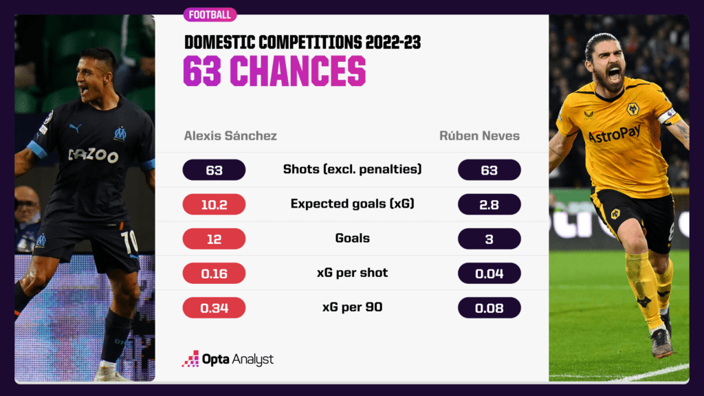
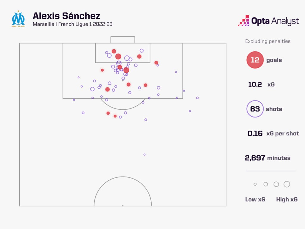
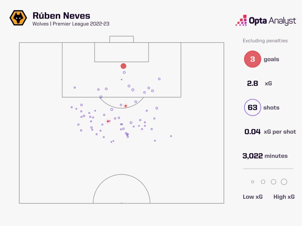
From the chances that Gabriel Jesus had we would expect the average player to score nearly 18 goals (17.7 xG). On the other hand, from Hakan Calhanoglu’s chances, we would expect the average player to score only 7 goals (7.0 xG). We can immediately understand why their goal scoring output was so different. Despite Jesus overperforming and Calhanoglu underperforming slightly according to their expected goals output, their 100 chances were very different in quality and their output reflected that.

We can compare the shot profiles of the two players by looking at their expected goals per shot (or xG per shot) which values the average quality of a player’s scoring chances. Gabriel Jesus’ xG per shot was 0.18, meaning that he would be expected to score approximately one goal for every five shots he took. The speculative nature of Calhanoglu’s shots resulted in a much lower xG per shot (0.07) that is evident in his shot map above, where the increasing size of the dot indicates an increasing xG value (and hence a higher likelihood of scoring).

We’ve focused on an individual player example here, but the expected goals metric can also be applied to teams or games in a similar manner. Of course, we can see here that a player or team may score more or less often than their xG value suggests but this is exactly the variance we can now analyse. Is a player scoring less than he should be? Who is getting chances from high xG situations?

Expected Goals Depth

Football is a relatively low scoring sport and so our ability to measure the likelihood of a goal being scored is essential context. With expected goals, we are arming pundits and analysts with another tool to quantify the stories that every football fan wants to hear. Which striker is struggling with their finishing? Which team’s form suggests they should be higher in the league table?

The unrivalled depth of Stats Perform’s data means that we now have over 2,500,000 shots enriched with xG values for more than 66,000 players that allows us to compare and understand performances of players and teams all over the world.

xG is a metric that goes beyond the traditional shot counts, but it is important to remember that it is still just a metric. We can use it to evaluate underlying performances, but it is the actual goals that are going to win you football matches. Football is unpredictable and goals can come from any number of unexpected outcomes but with expected goals, we can explain just how unlikely these were.